Computer Vision: Object Tracking

What is video analysis?

Video is just an ordered set of frames of the same resolution, where the frames are taken at regular time intervals. When constructing the video processing algorithm, we divide the video into two classes.

1. Video stream: is an ongoing video for online processing, where we don’t know the future frames.
2. Video sequence: is a video of fixed length and all frames are available at once, so we can process video sequence as a whole object.

What is optical flow?

Optical flow is a vector field of apparent motion of pixels between frames. Here motion field is the vector field of 2D projections of scene point motion vectors.

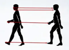
We can treat optical flow as estimation of the true motion field and this is one of the key problems in video analysis. What optical flow estimation means is it essentially is a pixel correspondence estimation problem, or a matching problem and can be regarded as a dense correspondence problem:

• Optical flow is a vector field ($u_{ij}, v_{ij}$) of apparent motion of pixels between frames.
• For each point ($x_{ij}, y_{ij}$) in first frame find a corresponding point ($x_{ij} + u_{ij}, y_{ij} + v_{ij}$) in second frame.

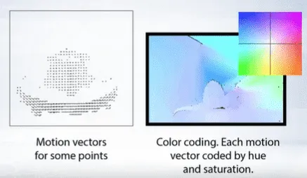
There are two main ways to visualize the result of optical flow estimation.

1. Directly draw motion vectors.
2. Color coding: For each possible motion vector, we specify a color.

Consider a pixel $I(x, y, t)$ and it moves by distance $(dx, dy)$ in the next frame taken after $dt$ time. Since those pixels are the same and intensity does not change, we can say,

Then by taking the taylor series approximation of the right hand side, removing common terms and dividing by $dt$ we get the following equation:

where

The above equation is called Optical Flow equation. In it, we can find $f_x$ and $f_y$, they are image gradients, similarly, $f_t$ is the gradient along time. But $(u, v)$ is unknown. We cannot solve this one equation with two unknown variables. So several methods are provided to solve this problem.

How do you solve the optical flow problem?

Lucas Kanade Method:

Optical Flow assumes that all neighboring pixels will have similar motion. Lucas-Kanade method takes a 3x3 patch around the point. So all the 9 points have the same motion. We can find $(f_x, f_y, f_t)$ for these 9 points. So now our problem becomes solving 9 equations with two unknown variables which is over-determined. A better solution is obtained with least square fit method. Below is the final solution which is two equation-two unknown problem and we can solve this to get the solution.

The idea is simple, we give some points to track, we receive the optical flow vectors of those points. But there are some problems. Until now, we were dealing with small motions, so it fails when there is a large motion. To deal with this we use pyramids. When we go up in the pyramid, small motions are removed and large motions become small motions. So by applying Lucas-Kanade there, we get optical flow along with the scale.

Dense Optical Flow:

Lucas-Kanade method computes optical flow for a sparse feature set. OpenCV provides another algorithm to find the dense optical flow. It computes the optical flow for all the points in the frame. It is based on Gunner Farneback’s algorithm.

The Gunner Farneback’s algorithm works as follows:

1. Take two frames
2. Approximate each neighborhood of both frames by quadratic polynomials using polynomial expansion transform
3. From observing how an exact polynomial transforms under translation a method to estimate displacement fields from the polynomial expansion coefficients is derived and after a series of refinements leads to a robust algorithm.

How do you evaluate the optical flow?

To evaluate the procedure of optical flow estimation, we need to compare estimated optical flow field and ground truth optical flow field. There are several metrics. Two of the most often used are

1. Angular error (AE): is the angle between estimated optical flow vector $(u_1, v_1)$ and ground truth optical flow vector $(u_0, v_0)$. It is measured as:

2. Endpoint error (EPE): is the distance between endpoints of estimated optical flow vector and ground truth optical flow vector.

Obtaining ground truth for optical flow is a very tricky problem because compared to image classification or object detection, we can’t just annotate image with human iterator. And we need to specify correct optical flow vectors for every pixel in the image. As a result, the number of available ground truth data for optical flow estimation is very limited.

How to use deep learning in optical flow estimation?

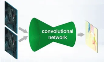
The straightforward way to use deep learning into optical flow estimation is to create a neural network that takes two frames as input and produce optical flow map as output. This approach was successfully proposed in FlowNet paper in 2015.

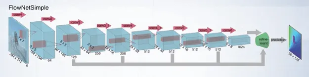
Two versions of FlowNet architecture was proposed.

1. Two color frames are concatenated into one image with six channels, instead of three. This image is then passed to the fully convolutional neural network.

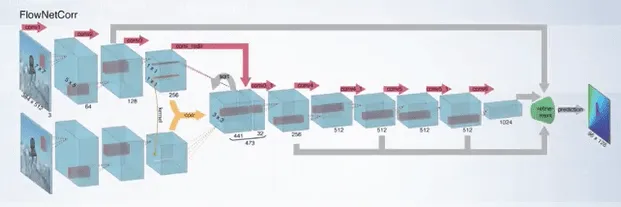
2. A siamese network is used. Two frames are separately passed through convolutional layers for feature computation. Then those features are then passed to a specific layer which implements patch comparison. It works similar to convolution, but without learnable parameters. In this layer, the dot-product between feature vectors for pixel in the first image and for pixel in the second image is computed. The results are passed next to the series of convolutional layers to estimate optical flow.

What is multi-scale pixel matching?

The dense matching of original input images can be broken down into set of simpler problems with multi-scale matching. First, we downscale input images. Then we apply dense matching to the downscaled version of input images, which is a simpler problem. For downscaled image, pixel displacement between images are shorter, thus the search space is smaller. The number of pixels in downscaled images are also much smaller. So we can apply complicated matching procedures that requires global optimization methods.

Then optical flow from downscaled images can be used as a starting point for optical flow estimation on original input images, which is much simpler than to try to estimate optical flow from original images.

In EpicFlow, edge-preserving guided interpolation is applied to sparse matches between images.

Guided upscaling of optical flow map can be performed by EpicFlow. But, in this paper, authors have additionally used homography based interpolation. For this, the image is first segmented and homography transformation is fit to semi-dense matches in each segment. If homography fits pixels of the segment well, then this segment has simple shape and upscaling is performed in this homography. Otherwise EpicFlow is used for this segment.

What is Visual Object Tracking?

Object tracking is the process of locating a moving object or multiple objects over time in the video. An output of object tracking is the object track. It is the sequence of object locations in each frame of a video.

Object to track is specified in the first frame of the video. We don’t know anything about an object except its location in the first frame, thus, object tracking is model-free tracking. We can’t build a detector to detect this object in other images. Because object appearance is changing over time, we consider only short-term tracking for this visual tracking problem in a short video sequences.

Challenges in developing a visual tracking method:

1. Computational Load: For each second of a video, we need to process a whole lot of frames.
2. Appearance change of the object over time. The appearance can change due to the object dynamics, viewpoint change, lighting change, and other reasons.
3. Object interaction: Other object can occlude the object of interest. The object appearance can be similar to other object.
4. Preparation of ground-truth data for visual object tracking is also a complicated process, but it’s easier than the optical flow estimation because human operator can usually track objects rather well, if not in real time.

Accuracy and robustness metric:

• Accuracy: average overlap during successful tracking
• Robustness: Number of times a tracker drifts off target
• Expected average overlap (EAO):
  • Re-initialization of tracker at overlap 0
  • Provides way to merge accuracy and robustness

Speed Metric:

• Equivalent filter operation (EFO): The idea is to reduce the hardware bias by reporting in tracking speed relative to the time required to perform filter operation. As a reference, take the MAX filter, it is applied in 30 by 30 window for all pixels in 600 by 600 pixel image. The time of tracking is then divided by the time of MAX filter.

What is model free tracking for visual object tracking?

In Model free tracking:

• We don’t know anything about object to track
• We can’t train object detector : In this regard, the usual tracking problem is similar to the image retrieval. In image retrieval, we rank images according to visual similarity of the probe image to the image in the gallery. In visual tracking, we search in the next frame for a region that is visually similar to the specified region in the first frame.
• Usually we build some description of object appearance, and search in next frame a region, similar to the object area in the first frame.

Object tracking works in iterative fashion. First, object model is initialized in first frame. Object models can be very different, but usually, the object is represented by a feature vector that describe object visual appearance as it is done in image retrieval. Then, starting from the position in the previous frame, we search in the current frame for a region which will be visually similar to the region in the previous frame. This can be done by sampling candidate regions in the neighborhood, computing feature vector for each candidate region and computing distance between candidate region and object model using the feature vectors. The sampling of candidate windows is similar to sliding windows in object detection. Measuring the visible similarity between images is similar to image retrieval.

Object representation in visual tracking:

• Object template: an example of instance of object of interest
• Object can be represented as a set of object parts or fragments of key points.
• Vector of appearance features: color histogram is an example

What is template matching?

• Take for example image of an object as a template t
• Now search for a new location of a template t in the next image f
• Then do a per pixel comparison of the template and image fragment with image distance metric (sum of squared distance) and Normalized Cross Correlation (NCC):

Visual tracking by pattern matching with normalized cross correlation is a baseline visual tracking method.

What is color based tracking for visual object tracking?

In Color based tracking: we can track object by color if object color is different from its surroundings.

To use color as a feature for tracking, you should estimate the likelihood of color sample to belong to objects or to the background. To do this,

1. Compute color histogram for the objects of interest inside the bounding box of the object.
2. Compute color histogram for the object neighborhood.
3. For each color value, compute likelihood ratio of the pixel to belong to object or to the background. This is an object background model.
4. Apply this model for each pixel in the current frame and segment a region that is highly likelihood pixels, or select a candidate region that maximizes object likelihood, or the sum of likelihood of pixels in this region.

Hue color object tracking is also regarded as a basic baseline method.

One of the key problems of color-based tracking is that the objects of interest can have similar appearance to other objects in the theme.

These objects are distractors for the visual tracking. Visual tracker tends to drift and can switch to tracking the similar objects. You can try to separate them directly. First, we need to detect distractors. So we apply object color model to the current image. Regions with high likelihood pixels are marked as distractors. Then, you compute color histogram for the distractor region. After that, it can estimate object likelihood at position X with respect to object color relative to the distractors. This will be object distractor model. We combine object background model with object distractor model in a linear combination.

Color based models are robust to object shape changes but sensitive to the blur and poor illumination. Template models rely on spatial configuration. So they are robust to blur and poor illumination but sensitive to changes in shape. By combining both features in a single model, you can make a tracker robust to both shape change and blur. Staple, or Sum of Template and Pixel-wise Learners is an example of such method.

What are the two ways to apply neural networks to visual tracking problem?

One way is to see it as a natural evolution of visual trackers and object detector simultaneously: We train convolutional neural network as object vs background classifier and apply it to the sampled candidate regions in the vicinity of the expected object position in current frame. The score of the classifier is a measure of visual similarity between candidate window and an object.

Eg: Multi Domain Network (MDNet tracker)-

• Train a neural network to distinguish object and background regions.
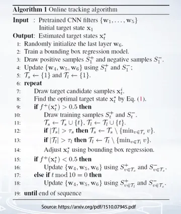
• Almost anything can be the object of interest, so we can’t train this network beforehand for all videos and for all type of object of interest : So we treat each video as a domain. Divide the neural network into shared and domain specific layers. We train the shared component offline on all available domains. Then, we train the domain-specific component for the target video online on the target video.

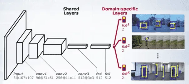
To improve the localization of object, a bounding box regressor is also trained for each domain-specific branch. Due to the complexity of the regressor, it is trained only once in the first frame of the video.

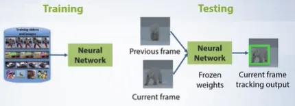
The second way is generic visual tracking: The idea is to train convolutional neural network that can regress the new position of any object which is positioned in the center of the previous frame. Such network takes two images as input. First image is the crop of the previous frame, centered at the object of interest. Second image is the crop of the current frame. The output is the new bounding box position in the current frame. Such network should be very fast because it doesn’t need online training.

Eg: Generic Object Tracking Using Regression Networks (GOTURN)

• Train a neural network using a collection of videos and images with bounding box labels.
• Apply this network at test time without fine tuning

The architecture of this network is similar to the patch matching networks used for stereo matching and optical flow estimation. But much larger images are taken as input.

1. Both images are parsed through a series of convolutional layers.
2. Outputs are parsed through a set of fully connected layers. The output to the net is bounding box of object in the second frame.

What is Multiple Object Tracking (MOT)?

There are two main differences between visual object tracking and multiple object tracking.

1. We need to handle multiple objects simultaneously.
2. Our goal is long term tracking instead of short term tracking.

There are two main variants of multiple object tracking problem.

1. Detection based tracking: when we have object detector and can apply to each frame in the video.
2. Detection free tracking: similar to visual tracking, we don’t know anything about objects of interest, except their bounding boxes in the first frame.

What is detection based tracking?

In detection based tracking:

• We specify a set of object classes we want to track. For each object, we should have a detector.
• The output of the multiple object tracking algorithm is the set of object trajectories or tracks for all objects detected individually.
• Object location in a frame is specified by the bounding box, the same as for object detection.
• MOT problem is an extension of object detection from single images to video. So, in addition to such object detection errors as false positive or false negatives, trajectory-specific errors are measured.
• ID switches occurs when for one ground truth object two trajectories are produced.
• Fragmentation occurs when for one ground truth object trajectory, two tracks are produced with a time gap between them. So, detections are missed in several frames.

There are several overall performance metrics, which are used simultaneously to measure the tracking performance:

• Multiple object tracking accuracy (MOTA) measures overall accuracy and the robustness of tracking. It measures total number of three types of errors; false negatives, false positives, and ID switch errors relative to the total number of ground truth detections individual. The best result is 1 or 100 percent.

• The multiple object tracking precision (MOTP) is the average dissimilarity between all true positives and their corresponding ground truth targets. It is computed as sum of bounding boxes overlap of target is assigned ground truth object to the total number of matches, thereby gives the average overlap between all correctly matched hypothesis in their respective objects and ranges between 50 percent and 100 percent.

What is object tracking by detection approach?

Object tracking by Detection Approach can be divided into two steps:

1. Apply object detector to each video frame or key-frames.
2. Associate these detections to tracks.

The typical problem of multiple object tracking is limited performance of object detector, it means detections and false positives.

Detection by tracking methods can be divided into two classes:

1. Online tracking, where only current and previous frames are available.
2. Offline or batch tracking, where all frames of video sequence are available.

The main part of tracking is association of detection between frames. Based on the number of frames in each particular step, you can divide methods into two frames and multiple frames methods.

In two frame methods, the associated detection in current frame is available tracks from the previous frame. In multi-frame methods, we consider a whole video or temporal window and we can change detection to track association for any frame in the window.

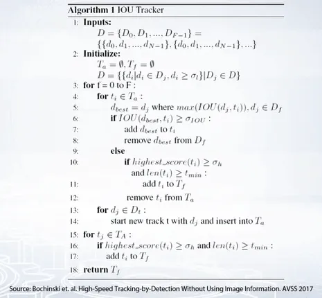
How do you evaluate object tracking by detection approach?

To associate detection and tracks, we need to estimate similarity or affinity between them. We can use several features to compute affinity score. Visual similarity, motion similarity and interaction between objects and objects within the scene are few examples. The simplest form of affinity is overlap between detection in the current frame and in the previous frame.

For each track, we select detection with the highest Intersection Over Union (IOU). If this IOU is larger than the threshold we add it to the track and remove it from the list of un-associated detections. If the best overlap is still lower than the threshold, we finish the track. If the track is too short or had no higher confidence detections we consider the track false positive and remove it from the final list of tracks.

If detector fails a frame and misses the object, then tracking of this object is stopped. False negative ID switch errors will be produced. The problem can be alleviated if it can use predicted object position instead of a missed detection in this frame. For example, we can use kalman filter to predict object position in current frame based on its position in previous frames. Then we can associate detections in current frame these predictions from previous frames. If object is not detected in the current frame, you don’t finish the track immediately but continue to track these predictions for several frames.

If predictions are good enough, we will successfully associate this detection with predicted position and assume tracking. Because predictions are less precise than detection, you should replace simple greedy based old methods with the optimal Hungarian algorithm for the assignment problem, as it was done in simple online in real time tracking.

Up till now, we haven’t considered object appearance and rely only on object motion. In this case, we can easily merge two tracks of different people if they move closer to each other. To add visual similarity to affinity cost, you can use imagery table method which is essentially a visual similarity estimation between images.

Addition of appearance similarity to affinity cost to this simple SORT algorithm, almost half the number ID switches and improves other parameters as well.

The detector and affinity score functions are two main components in multiple objects tracking methods. For both of these components, deep learning now demonstrate the best results. If we use a real time detector and the affinity estimate, then simple association method can be used in online tracking framework to achieve both real time performance and good tracking accuracy.

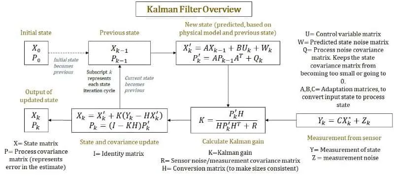
How does object tracking using Kalman filters work?

Kalman Filters, also known as linear quadratic estimation (LQE), is an algorithm that helps us to obtain more reliable estimates from sequence of observed measurements(sensor measurements). It can be used to track the position and velocity of a moving pedestrian over time and also measure the uncertainty associated with them. It is basically a two-step iterative process.

1. Predict: we predict the new position of a pedestrian based on the previous position assuming they are moving with a constant velocity.

2. Update: we take into account the actual measurements coming from the sensors to update our estimates. To do that we first calculate the difference between our predicted value and measured value and then we decide which value to keep by calculating the Kalman Gain. We then calculate the new value(new belief/position) and new uncertainty/error/variance based on our decision made by Kalman Gain. These calculated values will finally be the output of our Kalman Filter and will be used as an input to prediction step for next iteration.

Kalman Gain is a parameter which decides how much weight should be given to predicted value and the measured value. It checks the uncertainty in both predicted value and measured value and then it decides whether our actual value is close to predicted value or measured value.

A Kalman filter always works with linear functions. But most of the real world problems involve non linear functions. In most cases, the system is looking into some direction and taking measurement in another direction. This involves angles and sine, cosine functions which are non linear functions which then lead to problems. If we enter non-linear data in a Kalman filter, our result is no longer in uni-modal Gaussian form and we can no longer estimate position and velocity.

Extended Kalman Filter (EKF) proposes a solution to this problem. The EKF use Taylor expansion to construct a linear approximation of nonlinear function. We take mean of the Gaussian on the Non Linear Curve and perform a number of derivatives to approximate it. For every non linear function, we just draw a tangent around the mean and try to approximate the function linearly. Then we use that approximation as an input in our Kalman Filters equations to improve the accuracy of our position estimates.

Since here we approximate around only one point i.e. mean, the Gaussian we get doesn’t give us a good approximation.

Unscented Kalman Filter (UKF) proposes a solution to this problem. In UKF we have a concept of Sigma Points. Here we take some points (known as Sigma Points) on source Gaussian and map them on the target Gaussian after passing those points through some non linear function and then we calculate the new mean and variance of transformed Gaussian.

When a Gaussian is passed through a non linear function, it does not remains a Gaussian anymore but we approximate the Gaussian from the resulting figure, so in UKF a process called Unscented Transform helps us to perform this task.